Teaching

This page contains syllabi, problem sets, past exams, and other resources for the courses that I am currently teaching and have taught in the past.

Fall 2024: Graduate course on visualizations and GPU programming (AST3100)

In this course graduate students will learn the fundamentals of writing GPU accelerated parallel code and render scientific visualizations. No previous knowledge other than some basic programming experience (in any language) is required. During the course, students will be exposed to modern programming concepts and languages including WebGPU, HTML, JS, and WebAssembly which are very complimentary to what is typically used in purely scientific software. The skills learned in this course will be high valuable not only for students who wish to improve their scientific programming / visualization skills, but also for those who consider a non-academic career path. One goal of the course will be to create a dependency free visualization web-app from scratch that can run on many different operating systems. Each student will work on a project to visualize an astrophysical dataset (preferable a dataset they work on for their thesis) with the goal to make the visualizations publicly available.

Week 1

We went over the first example in the WebGPU fundamentals tutorial. Download the slides as pdf.

Week 2

We coded up this visualization of GAIA stars. Download the slides as pdf.

Week 3

Initial code.

WebGPU Editor.

Final code.

Lecture slides.

Week 4

Initial code.

Mid code.

WebGPU Editor.

Final code.

Lecture slides.

Week 5

WebGPU Editor.

Initial code.

Code after Task 1.

Code after Task 3.

Code after Task 4.

Code after Task 5.

Code after Task 7.

Code after Task 8.

Final code after Task 9.

Lecture slides.

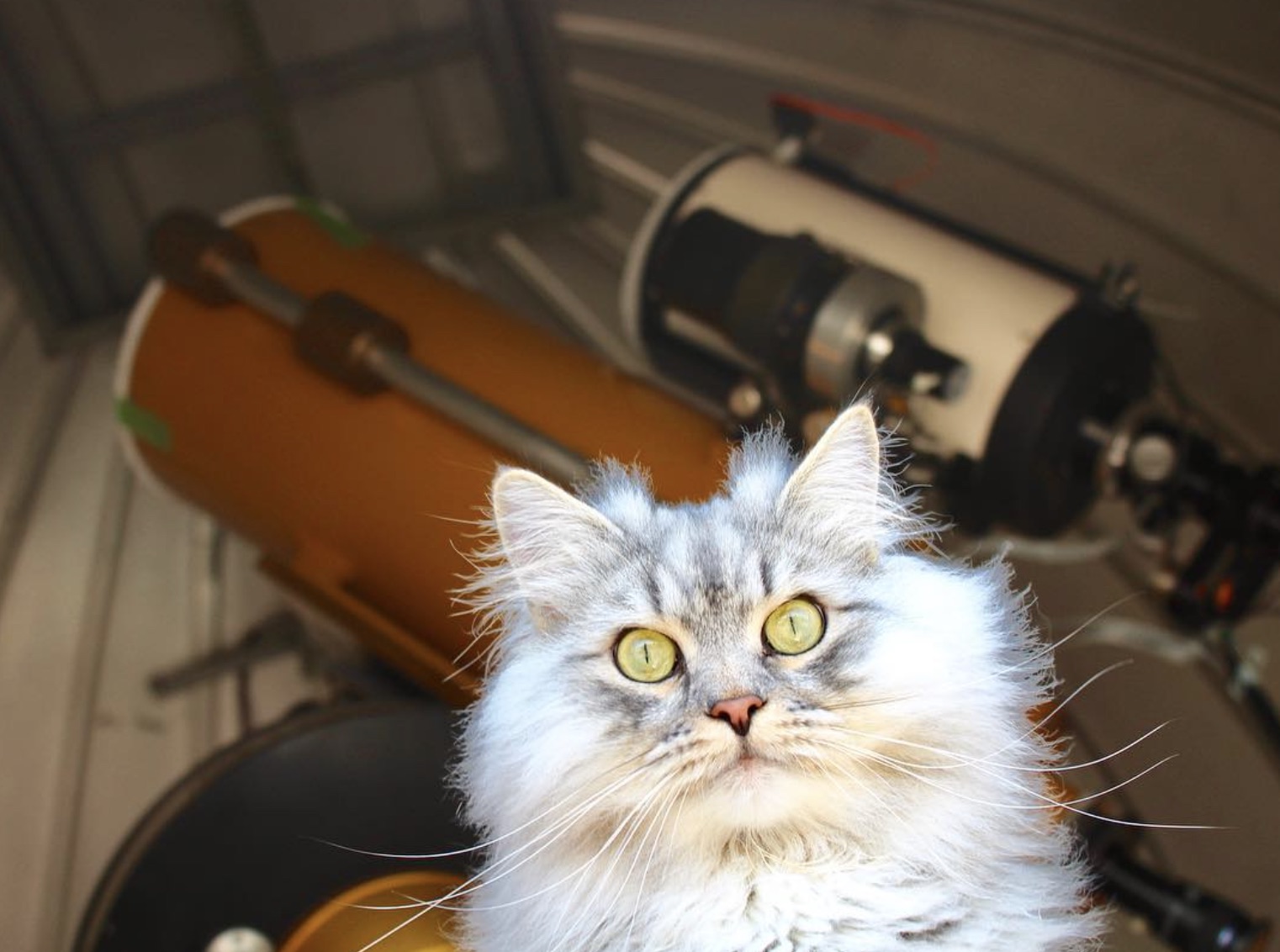
Puri Gagarin the Cosmocat visiting the UTSC Observatory.

Fall 2024: Practical Astronomy - Instrumentation and Data Analysis (ASTC02)

From the calendar: A hands-on introduction to astronomical observing using the UTSC telescopes. Lectures cover topics of astronomical instrumentation and data reduction. Observations of Solar System planets, moons, planetary nebula, globular clusters and galaxies will be made. Students will present their results in the style of a scientific paper and a talk.

Lecture notes week 1

Download as pdf.

Lecture notes week 2

Download as pdf.

Notebook for practical 2

Download as ipynb.

Notebook for practical 2 (simplified)

Download as ipynb.

Lecture notes week 3

Download as pdf.

Lecture notes week 4

Download as pdf.

Notebook for practical 3

Download as ipynb.

Lecture notes week 5

Download as pdf.

Notebook for practical 4

Download as ipynb.

Week 9

Popcorn timer.

Download lecture slides as pdf.

Lecture notes week 10

Download the Cosmic Distance Ladder part as pdf. Download as Stars part as pdf.

Lecture notes week 11

Download the slides as pdf.

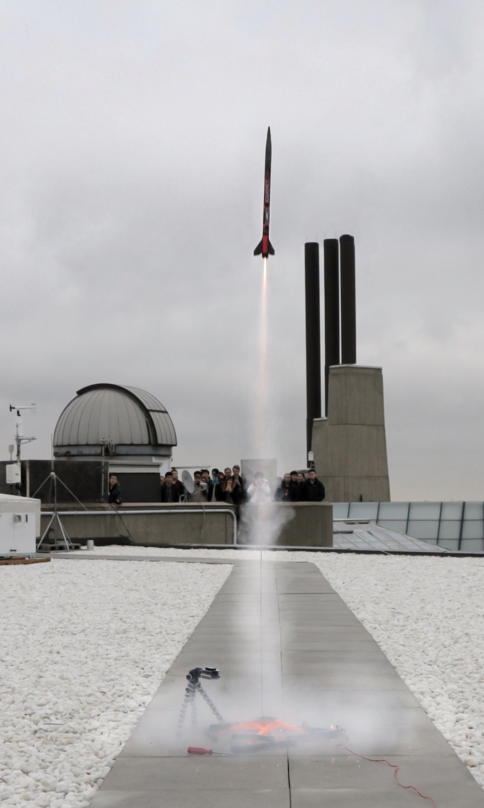
Launch of a rocket built by students in PHYB54 on the roof of the Science Wing.
(Winter 2024) Mechanics: From Oscillations to Chaos (PHYB54)

From the calendar: The linear, nonlinear and chaotic behaviour of classical mechanical systems such as oscillators, rotating bodies, and central field systems. The course will develop analytical and numerical tools to solve such systems and determine their basic properties. The course will include mathematical analysis, numerical exercises (Python), and demonstrations of mechanical systems.

Remote participation

Zoom. Password will be shared in the first lecture. You need to sign into zoom with your UofT account. You need to let me know before a lecture or tutorial if you plan to join remotely.

Introduction to python

This is a short tutorial on python, specifically intended for those who have no previous python or programming experience.

Reading for Lecture 2

Chapter 2.1 -2.6. Journal Questions:
  • What is the Reynolds number?
  • What is the terminal speed in a linear or quadratic medium?
  • Choose a random object from the same room as your are in right now. Guesstimate the characteristic drag timescale of the object as it moves through air!

Tutorial 2

Notebook from Tutorial 2.

Reading for Lecture 3

Chapter 3. Journal Questions:
  • Where is the centre of mass of the Earth Moon system (approximately)? Draw a sketch of the Earth Moon system in your journal (try to sketch it to scale, as best as you can)!
  • Which body contains most of the angular momentum in the solar system? Quantify!
  • Look up the specifications for an A8-5 rocket motor. Write down the thrust duration, the maximum thrust and the total impulse in SI units.

Tutorial 3

Notebook from Tutorial 3.

Reading for Lecture 4

Chapter 4. You do not need to read 4.6 and 4.7 very carefully. You may skip 4.5. Journal Questions:
  • What it the kinetic energy of the Earth going around the Sun (in kWh)?
  • What it the potential energy in the Earth-Sun system (in kWh)? Compare to the kinetic energy!
  • Come up with one explicit example of a position dependent force which is not conservative!

Tutorial 4

Notebook from Tutorial 4.

Reading for Lecture 5

First part of Chapter 5, from 5.1 to 5.4 (inclusive). Journal Questions:
  • Write down the general solution for the simple harmonic oscillator in four different ways: as a linar combination of two trigonometric functions, one trigonometric function with a phase, a linear combination of two exponentials, and as the real part of one exponential.
  • While your on a bus or in a car, try to estimate the frequency when you drive over a bump in the road. Also try to estimate if you are in a regime of over or underdamping.

Tutorial 5

Notebook from Tutorial 5.

Reading for Lecture 6

Second part of Chapter 5, from 5.5 to 5.8 (inclusive). No journal questions this week (I might still have your journal!). However, think about these two questions:
  • What is the differential equation for the driven, damped harmonic oscillator!
  • At what driving frequency does one get the maximum amplitude in a driven, damped harmonic oscillator? Write down the condition in terms of the natural frequency and the damping parameter.

Tutorial 6

Notebook from Tutorial 6.

Reading for Lecture 7

Chapters 7.1, 7.2, 7.3, 7.5, 7.7, 7.10. Journal Questions:
  • How is the Lagrangian defined?
  • Show that Newton's second law implies the Lagrange equations! (two line proof)
  • What are two major advantages of using Lagrange equations to solve problems in dynamics compared to just using Newton's laws?

Reading for Lecture 8

Chapter 8.1 - 8.6
  • What is the pericenter distance as a function of semi-major axis and eccentricity?
  • What is the relation between orbital period and semi-major axis?

Reading for Lecture 9

Chapter 11 (exclusive 11.7). Journal Questions:
  • Sketch the normal modes of a system consisting of two carts (Fig 11.1) where the masses of the two carts are equal and all spring constants are equal!
  • Sketch again the normal modes, but this time for a system where the oscillators are weakly coupled!

Tutorial 9

Notebook from Tutorial 9.

Reading for Lecture 10

Chapters 12.1, 12.2, 12.3, 12.4, 12.5. Journal Questions:
  • Write the equation of motion for the DDP in your journal!
  • Describe where the Feigenbaum number appears in the discussion of the DDP!
  • What is the Lyapunov exponent?

Tutorial 10

Notebook from Tutorial 10.

Reading for Lecture 11

Chapters 12.6, 12.7, 12.8, 12.9. Journal Questions:
  • What are the differences between a bifurcation diagram, a state-space orbit, and a Poincare section?
  • What is the recursion equation for the logistic map?

Lecture 11

Notebook from Lecture 11.

Tutorial 11

Notebook from Tutorial 11.

Old exams

Note that the format of this year's exam will be very different as it will be an open book exam.
  • Final exam from 2017. Download as PDF.
  • Final exam from 2018. Download as PDF.
  • Final exam from 2019. Download as PDF.
Puri Gagarin the Cosmocat visiting the UTSC Observatory.

Fall 2022: Practical Astronomy - Instrumentation and Data Analysis (ASTC02)

From the calendar: A hands-on introduction to astronomical observing using the UTSC telescopes. Lectures cover topics of astronomical instrumentation and data reduction. Observations of Solar System planets, moons, planetary nebula, globular clusters and galaxies will be made. Students will present their results in the style of a scientific paper and a talk.

Note that the course is currently scheduled as in person. Depending on the current state of the pandemic, the course might be switched to online synchronous for some or all of the lectures.

Please see Quercus for updates regarding this course.

Fall 2022: Introduction to Scientific Computing (PHYB57)

From the calendar: Scientific computing is a rapidly growing field because computers can solve previously intractable problems and simulate natural processes governed by equations that do not have analytic solutions. During the first part of this course, students will learn numerical algorithms for various standard tasks such as root finding, integration, data fitting, interpolation and visualization. In the second part, students will learn how to model real-world systems from various branches of science. At the end of the course, students will be expected to write small programs by themselves. Assignments will regularly include programming exercises.

Note that the course is currently scheduled as in person. Depending on the current state of the pandemic, the course might be switched to online synchronous for some or all of the lectures.

Please see Quercus for updates regarding this course.

Fall 2021: Introduction to Scientific Computing (PHYB57)

From the calendar: Scientific computing is a rapidly growing field because computers can solve previously intractable problems and simulate natural processes governed by equations that do not have analytic solutions. During the first part of this course, students will learn numerical algorithms for various standard tasks such as root finding, integration, data fitting, interpolation and visualization. In the second part, students will learn how to model real-world systems from various branches of science. At the end of the course, students will be expected to write small programs by themselves. Assignments will regularly include programming exercises.

Note that the course is currently scheduled as in person. Depending on the current state of the pandemic, the course might be switched to online synchronous for some or all of the lectures.

Please see Quercus for updates regarding this course.

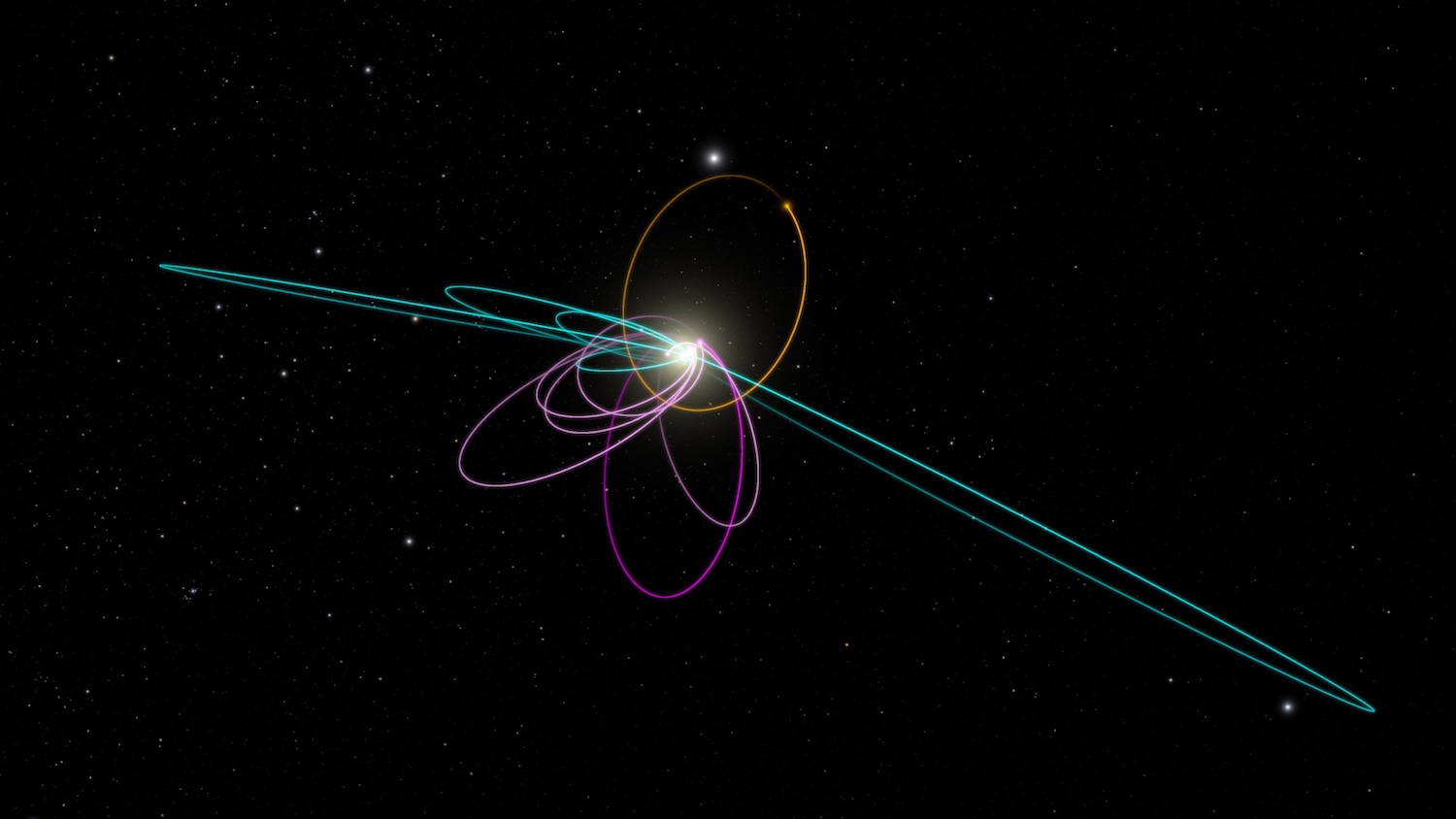
Planet 9 and Kuiper Belt objects (Caltech/R. Hurt/WorldWide Telescope)

Winter 2021: Planetary Dynamics (Graduate course, AST3100)

Since ancient times, humans have observed the night sky. One of the most striking feature easily observable with the naked eye are planets, the wandering stars. For centuries astronomers have recorded and predicted their motion. This course introduces graduate students to three topics in the wide field of Planetary Dynamics. Note that students can opt to take only one or two out of the three mini-courses being offered. But note that each mini-course builds on the knowledge developed during the previous mini-course(s).

You can download a tentative syllabus. If you would like to take this course, please get in touch via e-mail.

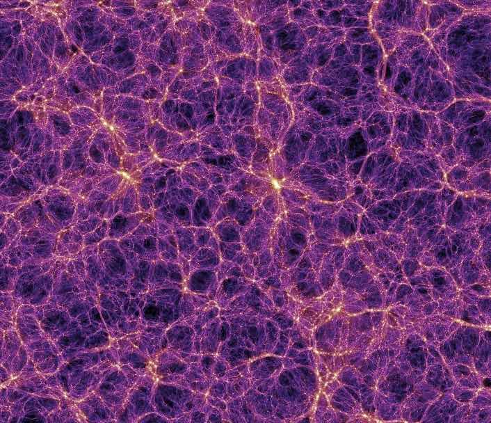
Simulation of the formation of large scale structure and galaxies in the early universe (Max Planck Institute for Astrophysics).

Fall 2020: Introduction to Scientific Computing (PSCB57)

From the calendar: Scientific computing is a rapidly growing field because computers can solve previously intractable problems and simulate natural processes governed by equations that do not have analytic solutions. During the first part of this course, students will learn numerical algorithms for various standard tasks such as root finding, integration, data fitting, interpolation and visualization. In the second part, students will learn how to model real-world systems from various branches of science. At the end of the course, students will be expected to write small programs by themselves. Assignments will regularly include programming exercises.

Please see Quercus for updates regarding this course.

Launch of a rocket built by students in PHYB54 on the roof of the Science Wing.
(Winter 2019) Mechanics: From Oscillations to Chaos (PHYB54)

From the calendar: The linear, nonlinear and chaotic behaviour of classical mechanical systems such as oscillators, rotating bodies, and central field systems. The course will develop analytical and numerical tools to solve such systems and determine their basic properties. The course will include mathematical analysis, numerical exercises (Python), and demonstrations of mechanical systems.

Syllabus

The syllabus includes a tentative schedule and the grading scheme. Download as PDF.

Introduction to python

This is a short tutorial on python, specifically intended for those who have no previous python or programming experience.

Tutorials

Note that the tutorials will be in SW505B.

Reading for Lecture 1

Chapter 1.1 -1.6

Reading for Lecture 2

Chapter 2.1 -2.6. Journal Questions:
  • What is the Reynolds number?
  • What is the terminal speed in a linear or quadratic medium?
  • Guesstimate the characteristic drag timescale of an every day object as it moves through air!

Reading for Lecture 3

Chapter 3. Journal Questions:
  • Where is the centre of mass of the Earth Moon system (approximately)?
  • Which body contains most of the angular momentum in the solar system? Quantify!
  • Look up the specifications for an A8-5 rocket motor. Write down the thrust duration, the maximum thrust and the total impulse in SI units.

Reading for Lecture 4

Chapter 4. You do not need to read 4.6 and 4.7 very carefully. You may skip 4.5. Journal Questions:
  • What it the kinetic energy of the Earth going around the Sun (in kWh)?
  • What it the potential energy in the Earth-Sun system (in kWh)? Compare to the kinetic energy!
  • Come up with one explicit example of a position dependent force which is not conservative!

Reading for Lecture 5

First part of Chapter 5, from 5.1 to 5.4 (inclusive). Journal Questions:
  • Write down the general solution for the simple harmonic oscillator in four different ways: as a linar combination of two trigonometric functions, one trigonometric function with a phase, a linear combination of two exponentials, and as the real part of one exponential.
  • While your on a bus or in a car, try to estimate the frequency when you drive over a bump in the road. Also try to estimate if you are in a regime of over or underdamping.

Reading for Lecture 6

Second part of Chapter 5, from 5.5 to 5.8 (inclusive). No journal questions this week (I have your journal!). However, think about these two questions:
  • What is the differential equation for the driven, damped harmonic oscillator!
  • At what driving frequency does one get the maximum amplitude in a driven, damped harmonic oscillator? Write down the condition in terms of the natural frequency and the damping parameter.

Reading for Lecture 7

Chapters 7.1, 7.2, 7.3, 7.5, 7.7, 7.10. Journal Questions:
  • How is the Lagrangian defined?
  • Show that Newton's second law implies the Lagrange equations! (two line proof)
  • What are two major advantages of using Lagrange equations to solve problems in dynamics compared to just using Newton's laws?

Reading for Lecture 8

Chapter 7.8. Journal Questions:
  • Who was Emmy Noether?
  • What is Noether's theorem?

Reading for Lecture 9

Chapter 8
  • How many orbital parameters do you need to describe the orbit of an asteroid orbiting the Sun? Make a list with symbols and names!
  • Sketch the orbit of Earth, Mars and the NASA InSight spacecraft! What is this type of orbit called?

Reading for Lecture 10

Chapter 11 (exclusive 11.7). Journal Questions:
  • Sketch the normal modes of a system consisting of two carts (Fig 11.1) where the masses of the two carts are equal and all spring constants are equal!
  • Sketch again the normal modes, but this time for a system where the oscillators are weakly coupled!

Reading for Lecture 11

Chapters 12.1, 12.2, 12.3, 12.4, 12.5. Journal Questions:
  • Write the equation of motion for the DDP in your journal!
  • Describe where the Feigenbaum number appears in the discussion of the DDP!
  • What is the Lyapunov exponent?

Reading for Lecture 12

Chapters 12.6, 12.7, 12.8, 12.9. Journal Questions:
  • What are the differences between a bifurcation diagram, a state-space orbit, and a Poincare section?
  • What is the recursion equation for the logistic map?

Assignment 1

Download as ipynb.

Assignment 2

Download as ipynb.

Assignment 3

Download as ipynb. Download initial conditions.

Old Final Exam from 2018

Download as pdf.
Simulation of the formation of large scale structure and galaxies in the early universe (Max Planck Institute for Astrophysics).
(Fall 2018) Introduction to Scientific Computing (PSCB57)

From the calendar: Scientific computing is a rapidly growing field because computers can solve previously intractable problems and simulate natural processes governed by equations that do not have analytic solutions. During the first part of this course, students will learn numerical algorithms for various standard tasks such as root finding, integration, data fitting, interpolation and visualization. In the second part, students will learn how to model real-world systems from various branches of science. At the end of the course, students will be expected to write small programs by themselves. Assignments will regularly include programming exercises.

Syllabus

The syllabus includes tentative schedule and grading scheme for the Fall 2018 term. Download as PDF.

Tutorial 2 Preparation

Check out this notebook to prepare for the test in tutorial 2.

Assignment 1

Download as PDF.

Lecture 1

Download the slides as PDF. The interactive part of the first lecture is based on this notebook (note that we did not cover all parts during the lecture).

Lecture 2

Video of Ariane 5 rocket launch. Lecture notes as a PDF.

Assignment 2

Download as PDF.

Lecture 3

Notebook of matplotlib and numpy introduction.

Assignment 3

Download as PDF.

Lecture 4

Lecture notes as a PDF.

Lecture 5

Assembler intepreter as a python file. Lecture notes as a PDF. Link to Micropython. Link to a description of the microcontroller board. Link to some of the sensors that you can use (I have also have other sensors not listed here).

Lecture 6

Lecture notes as a PDF. Python notebook on solving the heat equation.

Assignment 4

Download as PDF.

Lecture 7

Lecture notes as a PDF.

Midterm

Download the midterm (including solutions) as a PDF.

Assignment 5

Download as PDF.

Lecture 8

Lecture notes as a PDF.

Lecture 9

Lecture notes as a PDF. Slides on long term N-body integrations as a PDF. Python notebook and initial conditions for the N-body problem.

Lecture 10

Lecture notes on random numbers as a PDF. Slides on Bayes' Theorem as a PDF.

Lecture 11

For the various aspects of numerical integration we covered in the first 20 minutes of the lecture, see Computational Physics by Newman, chapter 5, which is freely available online.
Launch of a rocket built by students in PHYB54 on the roof of the Science Wing.

(Winter 2018) Mechanics: From Oscillations to Chaos (PHYB54)

From the calendar: The linear, nonlinear and chaotic behaviour of classical mechanical systems such as oscillators, rotating bodies, and central field systems. The course will develop analytical and numerical tools to solve such systems and determine their basic properties. The course will include mathematical analysis, numerical exercises (Python), and demonstrations of mechanical systems.

Syllabus

Includes tentative schedule and grading scheme for Winter 2018. Download as PDF.

Project

Outline for the ESP8266 project. Download as PDF.

Old exams

Midterm from 2017. Download as PDF.
Final exam from 2017. Download as PDF.

Driven Damped Pendulum

View the notebook from the March 29 lecture as a gist.

Slide from last lecture

View the slides from the last lecture as PDF.
Puri Gagarin the Cosmocat visiting the UTSC Observatory.

(Fall 2017) Practical Astronomy: Instrumentation and Data Analysis (ASTC02)

From the calendar: A hands-on introduction to astronomical observing using the UTSC telescope. Lectures cover topics of astronomical instrumentation and data reduction. Observations of Solar System planets, moons, planetary nebula, globular clusters and galaxies will be made. Students will present their results in the style of a scientific paper and a talk.

Syllabus

Includes tentative schedule and grading scheme. Download as PDF.

Github Repo

Various files for the tutorials and assignments can be found on the course's github repo.

Lab Report 1

Download the instructions for lab report 1 as a PDF file.

Lab Report 2

Download the instructions for lab report 2 as a PDF file.

Slides Lecture 1

Download the slides of lecture 1 as a PDF file.

Slides Lecture 2

Download the slides of lecture 2 as a PDF file.

Slides Lecture 4

Download the slides of lecture 4 as a PDF file.

Slides Lecture 5

Download the slides of lecture 5 as a PDF file.

Slides Lecture 6

Download the slides of lecture 6 as a PDF file.

Slides Lecture 7

Download the slides of lecture 7 as a PDF file.

Slides Lecture 11

Download the slides of lecture 11 as a PDF file.
Simulation of the formation of large scale structure and galaxies in the early universe (Max Planck Institute for Astrophysics).

(Fall 2017) Introduction to Scientific Computing (PSCB57)

From the calendar: Scientific computing is a rapidly growing field because computers can solve previously intractable problems and simulate natural processes governed by equations that do not have analytic solutions. During the first part of this course, students will learn numerical algorithms for various standard tasks such as root finding, integration, data fitting, interpolation and visualization. In the second part, students will learn how to model real-world systems from various branches of science. At the end of the course, students will be expected to write small programs by themselves. Assignments will regularly include programming exercises.

Submissions

To submit an assignment, go to portal.utoronto.ca.

Syllabus

Includes tentative schedule and grading scheme. Download as PDF.

Github Repo

Various files for the tutorials and assignments can be found on the course's github repo.

Geotab Project

Geotab project description with instructions and deliverables. Download as PDF.

Lecture Notes

Lecture 1

Introduction, floating point numbers. The following material is available: slides (pdf) and lecture notes (pdf).

Lecture 2

Floating point number boot camp and algorithmic complexity. The following material is available: slides (pdf) and solutions to the hand-out (pdf).

Lecture 3

Matricies, algorithmic complexity, LU decomposition. The following material is available: slides (pdf) and lecture notes (pdf).

Lecture 4

Review and examples for the linear least square fit (see handout from class), root finding algorithm, geotab walk through. The following material is available: lecture notes (pdf). The geotab example and the LU decomposition code are available as jupyter notebooks in the course repository on github.

Lecture 5

Root finding methods beyond bisection, gravitational wave discovery, plotting with matplotlib. The following material is available: lecture notes (pdf). The gravitational wave notebooks are available on the LIGO Open Science Center.

Lecture 6

Midterm, interpolation methods. The following material is available: lecture notes (pdf).

Lecture 7

Interpolation examples, introduction to differential equations. The following material is available: lecture notes (pdf), interpolation examples (github).

Lecture 8

Integration examples, N-body simulations. The following material is available: lecture notes (pdf).

Lecture 9

Numerical integration, Monte Carlo. The following material is available: lecture notes (pdf). Details on Buffon's Needle can be found on wikipedia. Details on random number generators and cryptography can be found in the Computational Physics book, chapter 10. A good introduction to Monte Carlo methods can be found in Helmut Katzbraber's lecture notes . In particular, read the chapter 2.2 on Markov Chains.

Lecture 10

Monte carlo methods, Bayes's theorem. The following material is available: slides (pdf).

Lecture 11

Quiz 4 (retake), review of material for the final exam. The following material is available: slides (pdf).

Lecture 12

Geotab presentations.

Final exams from previous years

Note that some content has changed! Download the 2014 exam as PDF. Download the 2015 exam as PDF. Download the 2016 exam as PDF.
Launch of a rocket built by students in PHYB54 on the roof of the Science Wing.

(Winter 2017) Mechanics: From Oscillations to Chaos (PHYB54)

From the calendar: The linear, nonlinear and chaotic behaviour of classical mechanical systems such as oscillators, rotating bodies, and central field systems. The course will develop analytical and numerical tools to solve such systems and determine their basic properties. The course will include mathematical analysis, numerical exercises (Python), and demonstrations of mechanical systems.

Syllabus

Includes tentative schedule and grading scheme. Download as PDF.

Problem Sets

Problem Set 1

Due: Monday, January 16th. Download as PDF.

Problem Set 2

Due: Monday, January 23rd. Download as PDF.

Problem Set 3

Due: Monday, January 30th. Download as PDF. Download solutions as PDF.

Problem Set 4

Due: Monday, February 6th. Download as PDF (updated 2017/2/3).

Problem Set 5

Due: Monday, March 6th. Download as PDF.

Problem Set 6

Due: Monday, March 13th. Download as PDF.

Problem Set 7

Due: Monday, March 27th. Download as PDF.
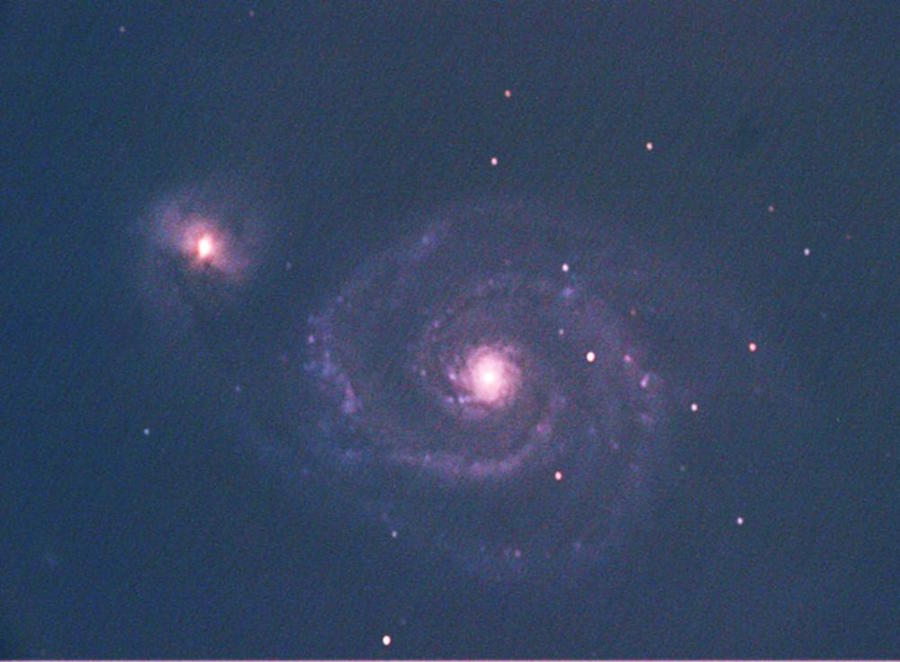
Image of M51 taken with the UTSC Observatory.

(Winter 2017) Galactic Structure and Dynamics (AST1420)

This is an introductory course to the galactic structure and dynamics. The course starts with discussing observational properties of star clusters, galaxies and galaxy clusters, before going into the mathematical details of modelling these systems. Assignments include numerical exercises.

Syllabus

Download as PDF.

Problem Set 1

Due: Tuesday, February 7th. Download as PDF.

Problem Set 2

Due: Tuesday, March 7th. Download as PDF.
Simulation of the formation of large scale structure and galaxies in the early universe (Max Planck Institute for Astrophysics).

(Fall 2016) Introduction to Scientific Computing (PSCB57)

From the calendar: Scientific computing is a rapidly growing field because computers can solve previously intractable problems and simulate natural processes governed by equations that do not have analytic solutions. During the first part of this course, students will learn numerical algorithms for various standard tasks such as root finding, integration, data fitting, interpolation and visualization. In the second part, students will learn how to model real-world systems from various branches of science. At the end of the course, students will be expected to write small programs by themselves. Assignments will regularly include programming exercises.

Submissions

To submit an assignment, go to http://rein.utsc.utoronto.ca/submit/.

Syllabus

Includes tentative schedule and grading scheme. Download as PDF.

Old exams

Note that the topics changed. For example, we did not do cover the assembler language this year.

Midterm

Download as PDF.

2014 Final exam

Download as PDF.

2015 Final exam

Download as PDF.

Assignments

Assignment 1

Python and Fibonacci numbers. Download as PDF.

Assignment 2

Floating point numbers, integers and computational complexity. Download as PDF.

Assignment 3

Linear least square fit. Download as PDF. Download climate data: climate.txt. Download solution: Solution_A3.py.

Assignment 4

Newton's methods, data files, bisection method. Download as PDF. (updated Monday Oct 24)

Assignment 5

Differential equations. Download as PDF.

Assignment 6

Your own project!. Download as PDF.

Lecture notes

Lecture 1

Introduction to Scientific Computing. Download slides as PDF. Floating point numbers. Download notes as PDF.

Lecture 2

Floating point number review, algorithmic complexity, matricies. Download as PDF.

Lecture 3

No lecture notes for this lecture. See Computational Physics by Newman, chapter 6.1. Code sample form the lecture: linearequations.py.

Lecture 4

Linear least square fit and root finding methods. Download as PDF.

Lecture 5

Root finding, interpolation. Download as PDF.

Lecture 6

Cubic spline, plotting, colour maps. Download as PDF.

Lecture 7

Differential Equations 1. Download as PDF.

Lecture 8

Differential Equations 2. Download as PDF.

Lecture 9

Monte Carlo. Details on Buffon's Needle can be found on wikipedia. Details on random number generators and cryptography can be found in the Computational Physics book, chapter 10. A good introduction to Monte Carlo methods can be found in Helmut Katzbraber's lecture notes . In particular, read the chapter 2.2 on Markov Chains.

Lecture 10

Numerical integration. See Computational Physics by Newman, chapter 5.

Lecture 11

Bayes' Theorem. See Think Bayes - Bayesian Statistics Made Simple